> For the complete documentation index, see [llms.txt](https://pop-lab.gitbook.io/bioinformatics-tutorials/llms.txt). Markdown versions of documentation pages are available by appending `.md` to page URLs; this page is available as [Markdown](https://pop-lab.gitbook.io/bioinformatics-tutorials/readme/mate-pair-links-in-metacarvel.md). # Mate-pair links in MetaCarvel ## Introduction Here we describe how links between contigs are managed in MetaCarvel. The basic idea is that paired reads generated by a sequencing instrument can be used to determine whether assembled contigs are adjacent to each other, as well as to estimate the relative position of the contigs along the chromosome being assembled. When multiple links occur between two contigs, MetaCarvel attempts to reconcile potentially inconsistent information such as different estimates of the relative orientation or positioning of the contigs. Here we provide an overview of the process used to process the mate-pair information and to resolve such inconsistencies. ## Overview of mate-pair use to link contigs First, a brief introduction to mate-pairs. A mate-pair is a pair of sequencing reads whose relative placement along a genome is approximately known. Depending on the technology used to generate such pairs of reads, this concept is also referred to as "paired ends", and, as technologies evolve, it is possible yet other terms will emerge to refer to the same type of information. To avoid confusion, we will only use the term "mate-pairs". 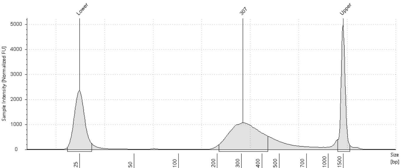### Fragment sizes Typically, the reads are paired, and occur within a certain approximately known distance, because they are both generated from a DNA fragment that has an approximately known size. The experiment used to generate fragments of an approximately known size yield a **library** of fragments, each of which is assumed to have a similar size. We typically assume the fragment sizes are drawn from a normal distribution characterized by a known mean (the target fragment size), and a standard deviation that depends on how precise the size selection process was. In reality, the distribution of fragment sizes is not normal, and skews towards longer fragments, as seen below.

Output from a DNA fragment size analyzer. The left-most and right-most peaks represent size standards (here with a known size of 25 and 1500 bp, respectively). The fragment library being analyzed is represented by the middle peak, with a mode at 307bp,but drawn from an asymmetric distribution with a longer upper tail.

We are not aware of situations in which modeling this distribution more precisely (than by approximating it with a Gaussian) yields substantially improved results, though we are also not aware of any studies specifically looking into this aspect of mate-pair bioinformatics. ### Read orientation Depending on the technology used to generate paired sequencing reads from a DNA fragment, the two reads may be generated from the same, or from complementary strands of DNA. Since each strand defines an implicit orientation when "reading" DNA, the two reads may, thus, have the same, or opposite orientations.

**Top:** Double-stranded DNA highlighting the opposite orientation of the two strands due to the 5'-3'unidirectional DNA replication process. **Bottom:** three possible scenarios through which a pair of reads (thick arrows labeled R1 and R2) can be derived from a double-stranded DNA fragment (thin long arrows).

The experimental protocol for creating mate-pairs results in the different relative orientations of the paired reads, and also impacts the way in which the original fragment length can be related to the actual placement of the reads in a genome sequence. For simplicity, we assume all read pairs are in an "innie" configuration (see below for other possible configurations).

Different types of relative orientations for the paired reads. For "innie" pairs, the fragment size is approximately the same as the distance between the furthermost ends of the reads.

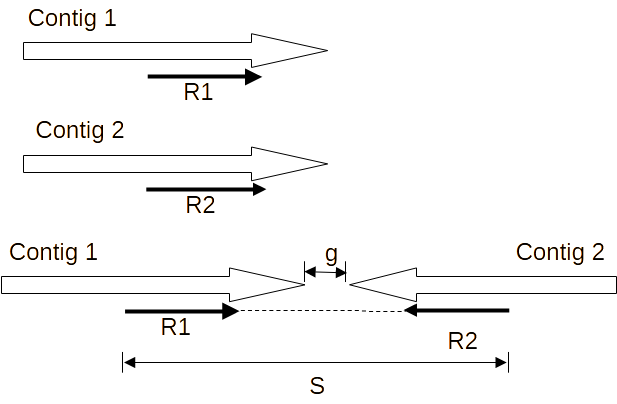
### From mate-pairs to relative contig placement To leverage knowledge about the distance between paired reads we need to know where these reads occur within assembled contigs. Such information may be provided directly by the genome assembler (though de Bruijn graph-based assemblers do not typically keep track of the reads), or has to be "reverse engineered" by mapping the reads to the assembled contigs. Once the placement of the reads within contigs is known, it becomes a matter of careful arithmetic to figure out what the paired reads tell us about the relative placement of the contigs. Of course, this information is only useful if the paired reads are aligned to different contigs. An example is provided below.

Two paired reads (R1 and R2) aligned to two different contigs (Contig 1 and Contig 2). In order to ensure the relative orientation and spacing of R1 and R2 are consistent with the sequencing experiment, contig 2 must be reversed (i.e., we infer it represents the complementary strand of the one from which contig 1 is derived). Furthermore, the gap g between the two contigs can be inferred from the size S of the fragment from which R1 and R2 are sequenced.

As can be seen from the picture, the (approximately) known relative placement and spacing of the paired reads implies the relative orientation and spacing of the contigs to which they align. The mathematical details of this inference will be described in more detail below. ### What comes next In the following sections we'll delve in more detail into the ways in which information about a mate-pair library is used in MetaCarvel to determine the relative placement of contigs within an assembly. Within this document we primarily focus on pairs of contigs, ignoring the broader context of the assembly graph that can be constructed from such pairs. The structure of the graph is impacted by genomic repeats (that induce links between contigs that are not actually nearby each other in the genome) as well as haplotype differences (that induce alternative paths through the graph) that occur between the paired chromosomes of eukaryotic organisms or between different organisms in a mixed sample (e.g., in metagenomics applications). ## Contig pairing estimation in detail Here we provide more detail about how mate-pair information is being used by MetaCarvel. At a high level, each mate-pair library (group of mate-pairs that derive from an individual sequencing experiment, and hence can be assumed to be drawn from the same size distribution) is processed separately, generating a collection of links between contigs. These links (across all libraries) are then "bundled" together to define the assembly graph. 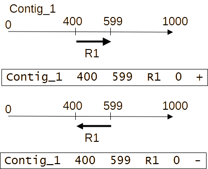### Determining the location of reads within contigs To determine the placement of reads within contigs, MetaCarvel relies on read alignment. While currently the tool relies on Bowtie2 \[to check], the actual alignment tool can be different as long as it can generate the information needed to create a [BED file](https://samtools.github.io/hts-specs/BEDv1.pdf). This type of file can represent the location of "features" along one or more chromosomes. In our case, each contig is a chromosome, and the features are the alignments of reads along the contig. MetaCarvel requires the first 6 fields of the BED format, specifically:

Col	BED field	Type	Description
1	chrom	String	Contig ID
2	chromStart	Int	Start coordinate of read alignment
3	chromEnd	Int	End coordinate of read alignment
4	name	String	Read name
5	score	Int	Currently ignored by MetaCompass
6	strand	String (+/-)	Read orientation (- means the read has opposite orientation to the contig)

Below are some examples of how this format translates to information about the placement of a read along a contig.

Two examples where read R1 (200 bp in length) aligns to Contig_1 (1001 bp in length). At the top, the read is aligned in the forward orientation, leading to the BED record listed below. At the bottom, the read is aligned in the reverse orientation.

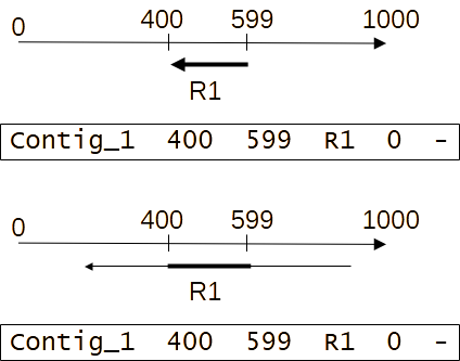
### Alignment pitfalls It is important to realize that it is possible for only part of the read to align to the contig, information that is not captured by the BED file. For example, in the example below, the BED records are identical, but the read at the top aligns fully while the read at the bottom only aligns partially.

BED record is the same even if only part of the read aligns (bottom example)

Thus, before constructing the BED file, it is important to filter the alignment and only retain those that represent nearly full-length matches, as they are most likely the actual locations of reads in the contigs. Also, it is possible for some reads to have multiple mappings. Some filtering needs to be put in place to retain the most likely position for every read, otherwise ambiguity will be introduced in the graph. It is important to realize, however, that some alignment tools only report one of the potentially many mappings, and may select an incorrect one. \[\* opportunity for further research] If only one of the paired reads has multiple mappings, it may make sense to create multiple links from the mate-pair, allowing later stages of the algorithm to resolve the ambiguity. If both reads have multiple mappings, the combinatorics may make such a process computationally prohibitive. 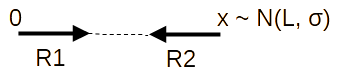### Translating coordinates Once we have the location of reads inside of contigs, we can start the process of using this information to determine the relative placement of contigs. To start, it is important to recognize that our primary reference is the mate-pair since the only (approximately) known information we have is the relative orientation and spacing of the two paired reads. Without loss of generality, we can assume that read R1 in a pair is in the "forward" orientation and that the coordinate of its leftmost end is 0. Given the known library size L and standard deviation $$\sigma$$, we can, thus, determine the location *x* of the beginning of read R2 as being drawn from a distribution with parameters (L, $$\sigma$$). Note that read R2 is in the "reverse" orientation, thus its start is the rightmost position in the diagram below:

Coordinates inferred from a mate-pair. By convention, R1 is in the forward orientation and anchored at 0.

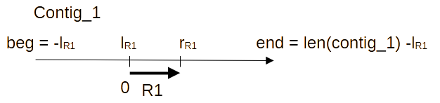
Let us now focus on just R1 and the contig that contains it (contig\_1). The BED file (described earlier) records the coordinates of the leftmost and rightmost positions of the read in the contig ($$l\_{R1}$$ and $$r\_{R1}$$) , as well as the relative orientation of the read and the contig. Let us first assume that the contig and the read are in the same orientation, and that the contig has length *len(contig\_1)*. The coordinates of the beginning (5' end, or *beg(contig\_1)*) and end (3' end, or *end(contig\_1)*) of the contig can now be calculated with respect to the new frame of reference anchored at the beginning of R1. $$ \substack{beg(contig\_1) = -l\_{R1}\end(contig\_1) = len(contig\_1) - l\_{R1}} $$

Computing the coordinates of the contig with respect to the read. Contig and read are both in the forward orientation.

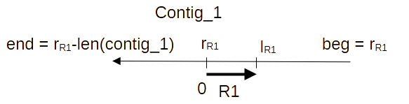
If the contig and the read have opposite orientations, then we have the situation in the figure below:

Computing the coordinates of the contig with respect to the read. Contig and read are in opposite orientations.

And the corresponding coordinates are: $$ \substack{beg(contig\_1) = r\_{R1}\end(contig\_1) = r\_{R1} - len(contig\_1) } $$ ### Building contig links In the previous section we saw how to compute the coordinates of the endpoints of a contig with respect to the frame of reference provided by one of the reads contained in the contig. Here we look at how this information translates into determining the relative orientation and distance between two contigs. 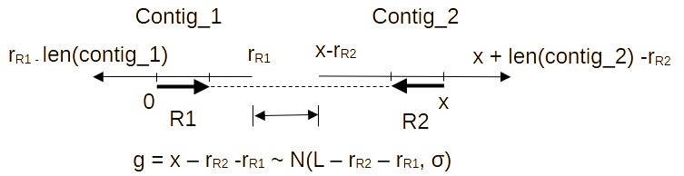Let us assume, for now, that R1 is contained in contig\_1 and R2 is contained in contig\_2, and that both R1 and R2 are in the opposite orientations with respect to their contigs. As seen in the figure below, the same type of arithmetic we used above can be used to compute the coordinates of the ends of the two contigs with respect to the start of R1. Thus, we can infer that the gap g between the beginnings of the two contigs is of length $$g=x - r\_{R2} - r\_{R1}$$ where x is drawn from a normal distribution representing the parameters of the sequencing library:

Computing a link between two contigs from the relationship between the paired reads R1 and R2.

Similar calculations can be performed for different relative orientations of the two contigs. Another way to think about this (and this is the way the code is actually implemented in Metacarvel) is to figure out how the mate-pair length *x* needs to be adjusted to generate a measurement of the gap between the contigs. As seen in the figure, we must subtract from X the distance between the beginning of each read and the corresponding beginnings of the contigs, or $$r\_{R1} + r\_{R2}$$. 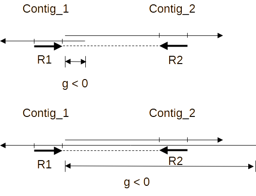### Contig linking pitfalls The drawing in the previous section highlights a particularly well-behaved case, where there is a gap between the two contigs. Below you can see some examples where the mate-pair information implies the contigs overlap, or even that one contig is contained in the other one.

Mate-pair information may indicate that the two contigs overlap (top) or one is contained in the other (bottom)

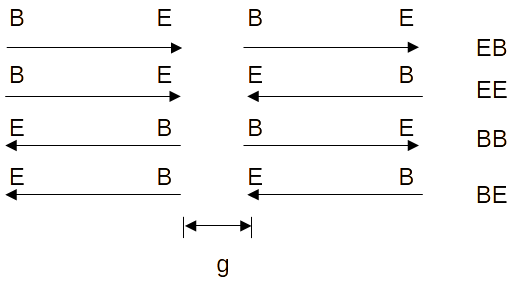
### Bundling contig links For every mate-pair that connects two contigs, MetaCarvel outputs a contig link in the format: ``` contig1 [TAB] (B/E) [TAB] contig2 [TAB] (B/E) [TAB] mean [TAB] stdev ``` where each field is TAB-delimited. contig1 and contig2 are the names of the adjacent contigs. Fields 2 and 4 indicate which ends (Beginning, or End) of the contigs are adjacent (see below), the mean is the mean size of the gap between the corresponding ends, and stdev is the standard deviation for the library.

Possible contig pairings. In all cases, the links reported by MetaCarvel include information about the size of the gap g, i.e., the distance between the named ends of the contigs.

Clearly, between any pair of contigs there can be multiple links. Since each link is processed separately, it is possible that the different links have different estimates for the relative placement of the contigs or the gap between them. Here we describe how such disagreements are resolved. First, for every pair of contigs, if the links imply different relative orientations, we process the links for each relative orientation separately, yielding a multi-graph that will be cleaned in later stages of the scaffolding code. 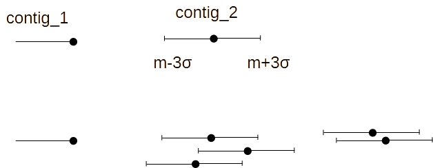At this point we can, thus, assume that all links imply a consistent relative orientation of the contigs. To resolve disagreements in length, we focus on the possible positions of the end of the second contig, assuming the end of the first contig is fixed. Since the gap size is related to the library size, which we assume to be derived from a normal distribution with mean *m*, we assume that the end of the second contig will occur with the confidence interval $$\[m-3\sigma, m+3\sigma]$$. To determine which links are compatible, we can now determine how the confidence intervals overlap (see below)

Top: confidence interval for the location of the end of contig 2, assuming the end of contig 1 is fixed. Bottom - multiple confidence intervals corresponding to different links between the two contigs. Groups of links where all confidence intervals share a segment are compatible. We retain the largest compatible group (here the one of the left with 3 links in it)

To determine which links generate similar (or compatible) relative placements of the two contigs, we find the links for which the confidence intervals overlap. In graph-theoretic terms, if we build a graph connecting two confidence intervals if they overlap, we are looking for a clique in this graph. While clique finding is generally NP-hard, since this graph is produced from interval overlaps (a special type of graph called an interval graph), this problem can be solved efficiently. The algorithm is essentially the same algorithm we use to compute the deepest depth of coverage within a contig (the place where most reads pile up on top of each other). Briefly, the algorithm works as follows: ``` Sort the starts and the ends of the confidence intervals together for each coordinate in the sorted list: if the coordinate is a start coverage += 1 if the coordinate is an end coverage -= 1 if coverage > maxCoverage: maxCoverage = coverage ``` The code shown above will compute the maximum coverage (or the maximum number of intervals that overlap each other). It is sufficient to modify the code to also remember which intervals were in the maximum pile-up. STOP AND THINK: The naive implementation can be quite expensive as you have to compute the list of overlapping intervals every time you update the maximum. Can you keep track of the list of intervals in the maximum clique efficiently? Once we've identified a list of compatible intervals, we can compute the combined estimate of the gap size as follows: $$ p=\sum{l\_i\over{\sigma\_i^2}} \ q=\sum{1 \over{\sigma\_i^2}} \ mean = {p\over q } \ stdev={1 \over \sqrt{q}} $$ where $$l\_i$$ and $$\sigma\_i$$ are the length and standard deviation of each of the links being merged, and mean and stdev are the mean and standard deviation of the combined "measurement". If all links are from the same library, thus all $$\sigma\_i$$ values are the same, the equations above simplify to: $$ mean = {{\sum l\_i} \over n} \ and\ stdev = {\sigma \over \sqrt{n}} $$ Where n is the number of links being combined and $$\sigma$$ is the library's standard deviation. \[Note: this idea for bundling when all links are compatible with each other was initially described by Huson and colleagues in ] Once the links are bundled, MetaCarvel outputs the contig "edges" in the following TAB-delimited format: `contig_1 [TAB] (B/E) [TAB] contig_2 [TAB] (B/E) [TAB] mean [TAB] stdev [TAB] nlinks` Where contig\_1 and contig\_2 are the contigs linked by an edge, the B/E fields indicate which ends of the two contigs are adjacent, mean and stdev represent the estimated size of the gap between the two ends, and nlinks indicates how many valid links are bundled together in this edge.